Standard Hyper Connections (HC) is unconstrained and said to be unstable for training. Manifold-constrained hyper connections (mHC) is an extension of HC that is empirically proven to be more efficient for training at scale.2 However with increasing model depth, mHC does not show consistent improvement to pretraining loss compared to HC, due to its constraining properties.1
Overview
The residual stream is an instrumental part of a transformer model. Residual connections are the pathways for transformers in which updates from transformer layers get accumulated. Residual connections provide a direct path for gradients, helping mitigate vanishing gradients in deep networks.4 There are two types of residual streams - PreNorm & PostNorm. PreNorm is more commonly used as it serves as a good optimization technique and allows clean differentiation of gradients during backprop. However, the magnitude of the residual stream gets very large every layer relative to individual layer updates. This causes deeper layers’ updates to dilute and become less effective.
Read more from my notes on residual methods here.
For better depth utilization, ByteDance introduced Hyper Connections3, which is a redesign of the residual stream. HC widens the residual stream by having many parallel residual streams at once. These parallel streams are then aggregated into a single input before entering attention/ffn layers, and then expanded back to parallel streams again before applying an $n \times n$ map (a cross-stream mixing matrix) for mixing information across streams.
However these $n \times n$ maps can cause training instability as they are unconstrained matrices, and can therefore grow/shrink throughout training. mHC2 solves the training instability by constraining the $n \times n$ map to a manifold.
These methods work well for regular training so far. But recent research (DepthBench1) found that mHC’s benefits don’t translate for deeper models.
Following this paper, I wanted to experiment and compare HC against mHC at 3 different aspect ratios at a much smaller scale on a modded-nanogpt baseline, to see how the effective ranks are affected over training. More on the setup below.
Hyper Connections:
Hyper connections were introduced to boost residual capacity by adding more parallel residual streams. To allow the streams to share information with each other, they introduce an $n \times n$ matrix $H_l^{\mathrm{res}}$ which exchanges / mixes information before the layer update.
Before the attention or feedforward layers, the residual streams are aggregated into a single input since these layers cannot handle wide residual shapes.
To better understand this let’s backtrack a bit to standard residual connections and see what it’s doing:
$$x_{l+1} = x_l + F_l(x_l)$$
It adds layer updates into a single residual stream.
But now with hyper connections, we have $n$ parallel residual streams
$$X_l = \begin{bmatrix}x_l^{(1)} \\ x_l^{(2)} \\ \vdots\end{bmatrix}$$
so the update becomes:
$$X_{l+1} = H_l^{\mathrm{res}}X_l + H_l^{\mathrm{post}}F_l(H_l^{\mathrm{pre}}X_l)$$
what res mapping, pre and post mapping mean:
- $H_l^{\mathrm{res}}$ → mixes information between the parallel residual streams
- $H_l^{\mathrm{pre}}$→ reads all $n$ residual streams into a single matrix input before the layer. Also uses a sigmoid function to maintain non-negative values to keep the values from cancelling each other out
- $H_l^{\mathrm{post}}$ → broadcasts back the layer output into its $n$ parallel residual streams. This also maintains non-negative values.
the $H_l^{\mathrm{res}}$ matrix is a square matrix. the singular values of this matrix are unconstrained and can therefore blow up or vanish across layers, making training very unstable. mHC fixes this.
Manifold-constrained Hyper Connections (mHC)
To prevent the $H_l^{\mathrm{res}}$ from exploding or vanishing singular values, mHC enforces a geometric constraint to the matrix by projecting $H_l^{\mathrm{res}}$ to the Birkhoff polytopeBirkhoff polytope is the set of all n×n doubly stochastic matrices. It runs the Sinkhorn-Knopp normalization on $H_l^{\mathrm{res}}$ to make it doubly stochastic.
A doubly stochastic matrix is when both the rows and the columns sum to 1.
But how does a doubly stochastic matrix ensure stable training?
It preserves the norm of the matrix. In a doubly stochastic matrix, the matrix is essentially a convex combination of the inputs. (convex combination is just a weighted average where the weights are non-negative and add to 1).
For example: if $H_l^{\mathrm{res}}$ is
$$H_l^{\mathrm{res}} = \begin{bmatrix}0.3 & 0.7 \\ 0.7 & 0.3\end{bmatrix}$$
then
$$0.3x_1 + 0.7x_2$$
if $x_1 = 10$ and $x_2 = 20$, then
$$0.3(10) + 0.7(20) = 17$$
which lies between 10 and 20.
Another thing is that the product of doubly stochastic matrices is also doubly stochastic. Which means that its stability persists across depth.
This is how mHC constrains outputs across layers and ensures it does not blow up.
Constraining makes matrices low rank
The rank of a matrix is the maximum number of linearly independent rows or columns in a matrix, which tells us how much unique information is stored in that matrix. For richer representations in the residual stream, we want matrices to have higher rank.
The matrix of interest here is $H_l^{\mathrm{res}}$, the cross-stream information mixing matrix that mHC constrains. Since Sinkhorn–Knopp normalization is repeatedly applied to the matrix, forcing the row and col to sum to 1, over many layers this gradually compresses the matrix to become low-rank uniform distribution. Therefore the rich parallel residual streams end up collapsing into a single homogeneous stream.
What this means for computational depth
mHC over-constrains the $H_l^{\mathrm{res}}$ matrix across layers and this causes all unique residual paths to collapse into one identical path. mHC’s products across layers have much lower effective rank compared to HC, reducing deeper layers’ effectiveness. HC on the other hand is unconstrained, and preserves the rank of the matrix throughout training, allowing the deeper layers to be more effective with additional computational depth.
HC vs mHC
In a small experiment I ran I compared the performance of HC and mHC over 3 different aspect ratios (to keep the setup iso-param) on a modded-nanogpt baseline. Full code for the experiment can be found here.
Similar to results in the DepthBench1 paper, mHC reduces effective rank across training. You can see visually in this plot below, mHC has lower effective rank at deeper layers.

side note: deep narrow mHC run stopped due to resource constraints. but the trend as seen in the val loss still holds the claims.
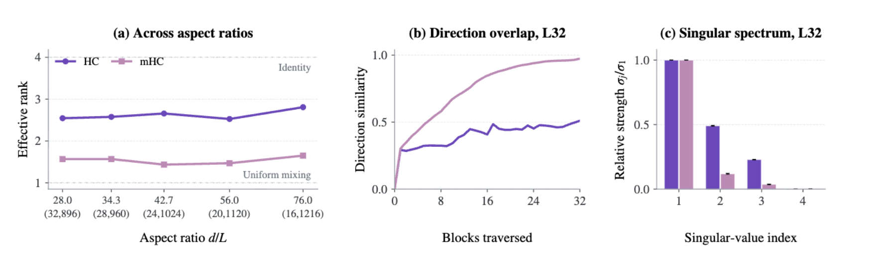
This confirms the results in DepthBench1, where HC's residual transport retains higher effective rank than mHC's with deeper/narrower models.
HC's lower validation loss isn’t too surprising since these are small runs. DeepSeek's mHC paper2 motivates its constraints with training instability that is observed at much larger scale ( 27B model / 60+ layers). HC did not show any instability in the runs above. Meanwhile, mHC’s residual transport still lost effective rank across depth.
Discussion
The takeaway is that while manifold regularization (mHC) can prevent vanishing or exploding gradients during large scale training, it aggressively constrains matrices to the Birkhoff polytope, causing the residual stream’s representational diversity to decrease across depth. Computational depth research would benefit from better residual stream designs that have the same training stability as mHC but can also preserve the rich residual stream and effective rank as HC.