How to Build a Brain (without losing yours): Intro to Neuromorphic computing
With frontier labs like OpenAI investing billions on compute, third generation energy efficient neural networks that are developed to closely mimic human brain are becoming more and more relevant.
I went deep into a neuromorphic computing rabbit hole recently and so this blog is an attempt at documenting everything I learnt and read about it. The goal is to be able to build a minimal brain-inspred model that is power efficient and can classify images. I’ve skipped the math and have written from an intuitive sense, with some code snippets. You can find the full code in my GitHub.
In this blog I cover:
- how the brain works from a neuroscience perpective
- training SNN on the mnist dataset
- calculating power efficiency of the model
- why do SNNs work
- neuromorphic hardware
Let’s start!
The human brain, and why it's efficient
First, some terminology:
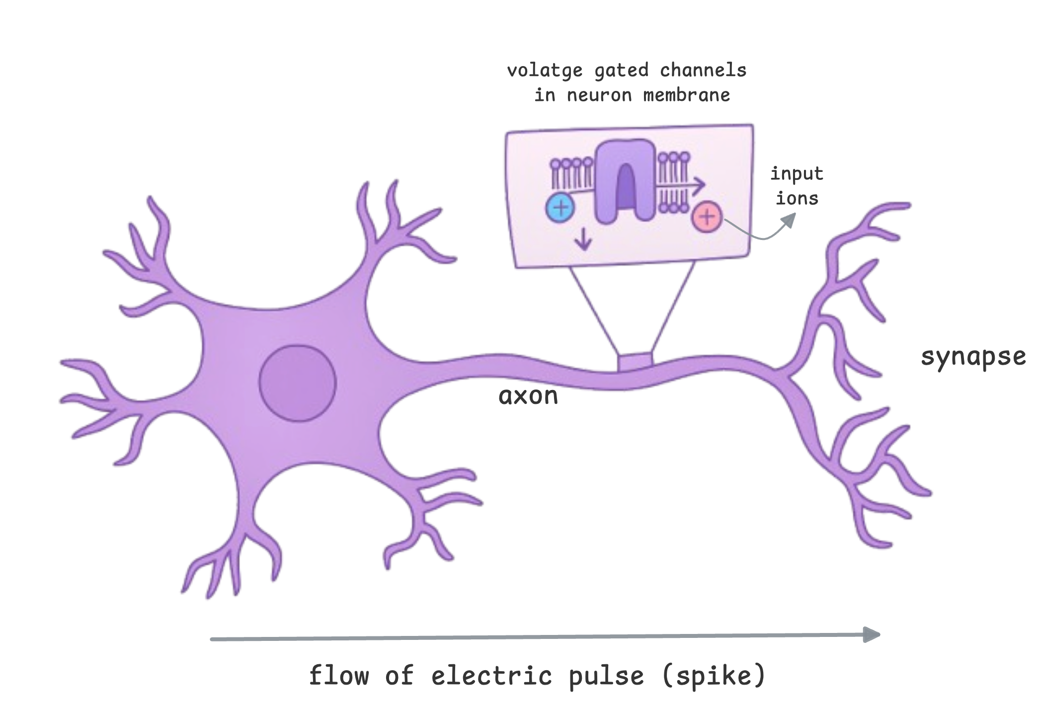
- membrane - walls of the axon
- membrane potential - electric voltage in a neuron's membrane
- spike - electrical pulse sent to the next neuron when membrane potential crosses a threshold
- synapse - gap between two neurons (SNNs use synaptic weights)
- synaptic strength - how much influence one neuron has on the next
- synaptic plasticity - property where synapses change their strengths over time
Biological neuron computations are temporal. If you are a human reading this blog, you don’t just see this blog as a static chunk of tokens. Your brain processes motion, changing contexts, sequence of sounds etc. and the timing of your neuronal responses impacts how you perceive the environment around you.
Brains process information through discrete electrical impulses called spikes (aka action potential as biologists say). When a neuron in your brain fires, its called a spike. Everything we see and perceive is a spike.
Example: when you listen to music you like, your ears convert them into spike trains, accumulates spikes over time, recognizes spike patterns and classifies it. (happens very very quick)
So,
Exciting stimulus → voltage gated channels along the membrane open → ions mass flow across membrane → ion concentration in neuron accumulates → membrane potential increases → reaches threshold → neuron spikes & fires → electric pulse / signal sent to neighboring neuron.
I like to think of passing electric signals down to neurons as an eqivalent to a feed forward.
Here is a live interactive simulation:
Controls
Press & hold to stimulate.
Live Stats
This is exactly what we are trying to copy here. We want to be able to accumulate inputs over time, and fire when it reaches a threshold. The Leaky Integrate and Fire (LIF) neuron does exactly that.
The reason for biological brains being very energy efficient is that the synapse merges both memory storage and data transfer, so it doesn’t waste energy shuttling data. Also, neurons activate & perform computations only when they have something meaningful to say, which is when its membrane potential reaches threshold and spikes. As opposed to traditional neural nets, where every neuron performs dot product in every forward pass, whether it conveys meaningul information or not. And every dot product computation eats up some energy.
Spiking Neural Networks
Neuromorphic computing is both a hardware and software problem. We need an algorithmic side to perform event driven computations, in a dynamic way the brain does. The main differentiator between spiking neural nets and regular neural nets is the time dimension that helps accumulate inputs.
Best way to learn is by doing. So in this blog let’s train a spiking neural net on the famous MNIST dataset to classify digits. You don’t need any neuromorphic hardware for this implementation, it can be done on a cpu.
Just a disclaimer that all the numbers in the diagrams are random placeholder values. It’s just to show how data flows through the network.
Spike Encoding a static dataset
Like any ml project, first we need to prepare our dataset.
The MNIST dataset is a static dataset… because each image is just a 2d grid of static pixel values, and have no aspect of time or motion. Biological neurons however process all sensory input as spikes over time. So before feeding the mnist dataset into a spiking neural network, we need to give these images a time dimension by converting each pixel intensity into spike trains.
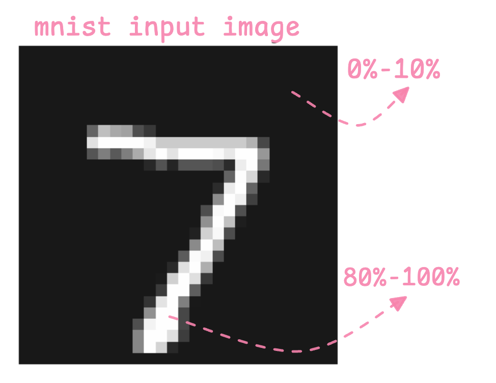
This is called rate encoding - where we encode each pixel into a spike train. Say we have an input image of the number 7, the surrounding pixels are darker and have lower intensity (~0%-10% brightness), and the pixels making up the number are brighter and have higher intensity (~90%-100% brightness).
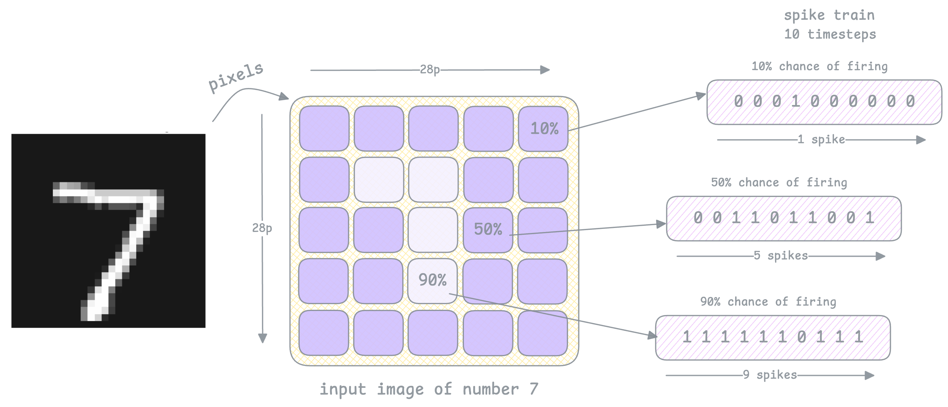
Rate encoding treats each pixel's intensity value as a spike probabilty per timestep, using bernoulli trials.
So over 10 timesteps (for example):
- a white pixel (value 1.0) → spikes mostly 10 out of 10 timsteps
- a grey pixel (value 0.6) → spikes about 6 out of 10 timesteps
- a dark pixel (value 0.1) → spikes about 1 out of 10 timesteps
It defines how many times spikes accumulates. Usually its better to give longer timesteps for better approximation of spike rates.
This is how we can encode the image into spike trains:
In other conventional netoworks like ANN, the input image would just be flattened into a scalar input vector and sent through a forward feed network.
The spikes are the reason behind energy efficiency because they are binary events, it either spikes (1) or not (0). Since these input spikes trains are sparse, mostly 0s, it is easy to multiply and cheap to store.
This line of code uses snnTorch's spikegen.rate function to rate encode inputs:
spikedata = spikegen.rate(data.view(data.size(0), -1), num_steps=timesteps)
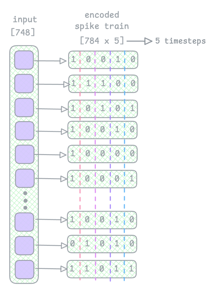
There are 28 * 28 = 784 pixels in an mnist image. If we encode each pixel into a spike train, we get 784 spike trains, one for each pixel.
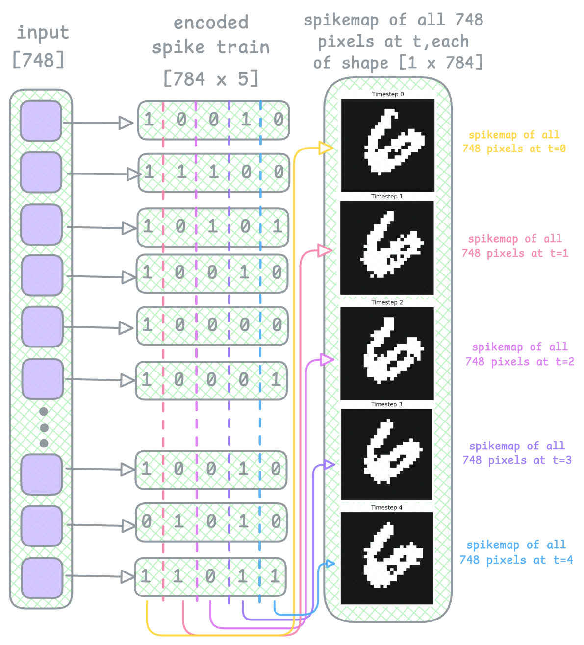
After encoding, here is a spike map at each timestep, that shows which of the 784 pixels of the input image spiked at that timestep, and you can see that rate encoding made sure pixels probabilistically spiked where the bright pixels are:
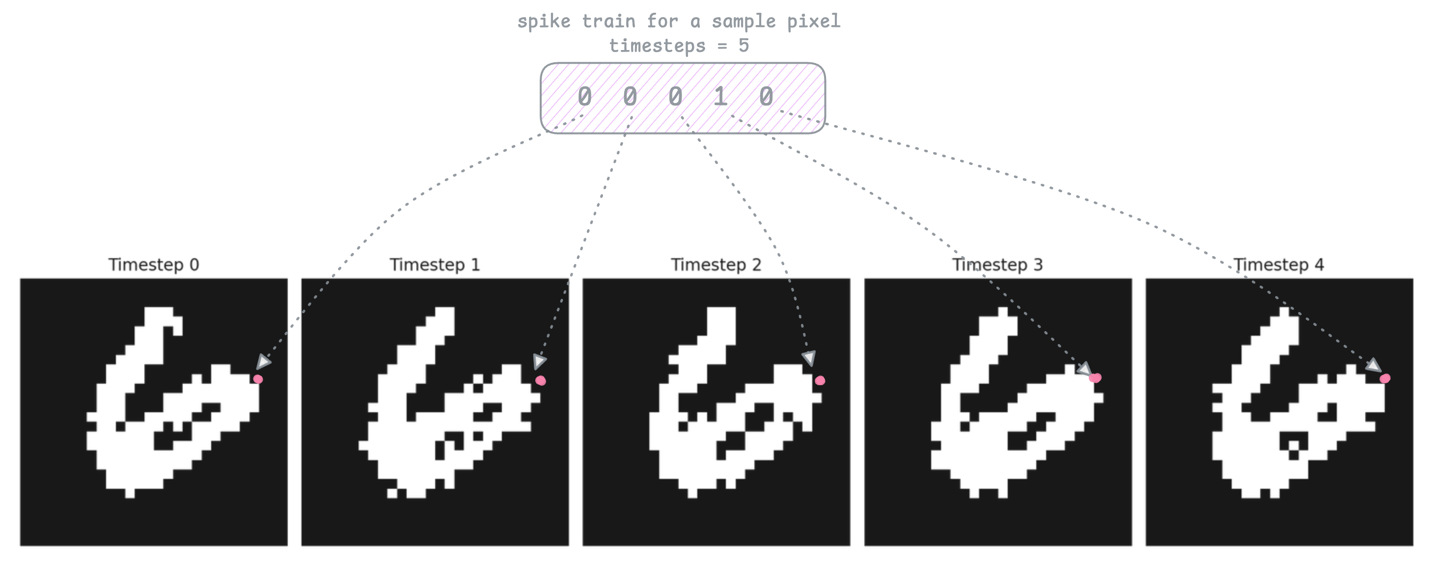
In the image above I marked the particular pixel for this example. The spike train above shows that the same pixel spiked 1 out of 5 timesteps.
Just to be clear, these are not the input images. There are no grey pixels here like in the original mnist images. These maps are just black/white squares representing the spikes at each timestep. After encoding all images of our dataset, we pass in these maps into our feed forward netowork as inputs. Each spikemap is actually passed into the network seperately as a [1 x 784] shaped vector with 0s denoting black squares, and 1s for the white squares.
As an alternate to rate encoding I have also seen a few methods where you can just pass in the same static image as input for every timestep, instead of a spike train of len(timesteps). But this is not what happens in the brain and is less preferred.
Leaky Integrate and Fire Neuron
A simple LIF neuron,
- accepts input spikes from previous neurons
- accumulates them as membrane potential
- leaks accumulated potential if there's no new input
- reaches a pre-defined threshold value
- sends a spike (1) to the next neuron
- resets back to resting potential
and this process repeats for len(timesteps)
You can try the interactive simulation from earlier again to see this in action.
Think of a neuron like a leaky bucket:
- Every incoming spike adds a little water (charge).
- The bucket has a hole, so water slowly leaks out.
- If enough water comes in fast enough → the bucket overflows → the neuron fires a spike.
- After firing, the bucket resets to empty, and the process repeats.
So to cause this "overflow", we need strong enough or exciting inputs to reach the threshold faster. The leak makes sure old inputs go away, and only new inputs matter, creating a temporal filter.
So for our MNIST dataset, brighter pixels have higher probability of spiking, so they produce spike trains with more spikes. For this reason when these input spike trains are passed into the network, the LIF neurons accumulates brighter pixels faster and generates output spikes more frequently.
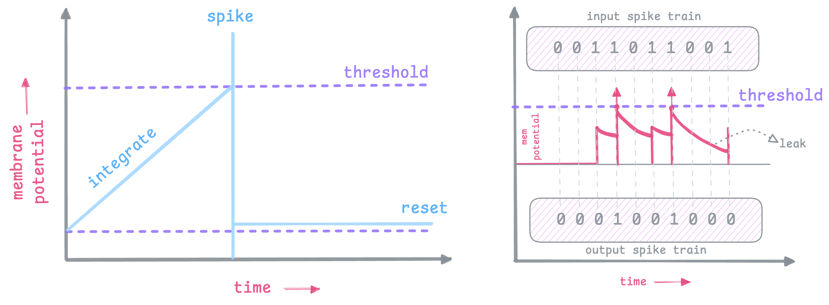
As you can see in the diagram, as the input integrates (and leaks), once it reaches threshold, an output spike is generated.
snnTorch beautifully abstracts this for us, but this is what LIF neuron looks like as a function:
    def lifneuron(mem, spike, thresh=2, tau=20.0):
        leak = -mem/tau # how much to leak
        mem += leak + spike # integrate mem potential with leak
        spk = (mem >= thresh).float() # checking if mem potential crossed threshold
        mem *= (1 - spk) # reset mem potential if spiked, multiply mem by (1 - spk)
        return mem, spk # Return updated mem potential and output spike
Network Architecture
Now we will put together a simple network. The example implementation from snnTorch uses this same network, and so I will be explaining this, but feel free to experiment with the hyperparameters.
As you can see in the code snippet below, we define 4 layers:
Hidden Layer
- fc1 → a fully connected learnable weights
- lif1 → spiking neuron layer that acts as an activation layer
Output Layer
- fc2 → second fully connected learnable weights
- lif2 → spiking neuron layer
The fully connected layers have the weight parameters that the model learns and the lif layer does the spiking temporal behaviour.
class snNet(nn.Module):
    def __init__(self):
        super().__init__()
        self.fc1 = nn.Linear(num_inputs, num_hidden)
        self.lif1 = snn.Leaky(beta=beta)
        self.fc2 = nn.Linear(num_hidden, num_outputs)
        self.lif2 = snn.Leaky(beta=beta)
snn.Leaky creates the LIF neuron layer, and beta is rate of 'leak' we spoke about earlier. You want to find a sweet spot for beta, usually:
beta = 0means that the neuron will not have any memory, favors most recent input and forgets the previous inputsbeta = 1means the neuron will accumulate all inputs and there is no leak happeningbeta = 0.9is a sweet spot for me and shows slight leak/decay
Forward Pass
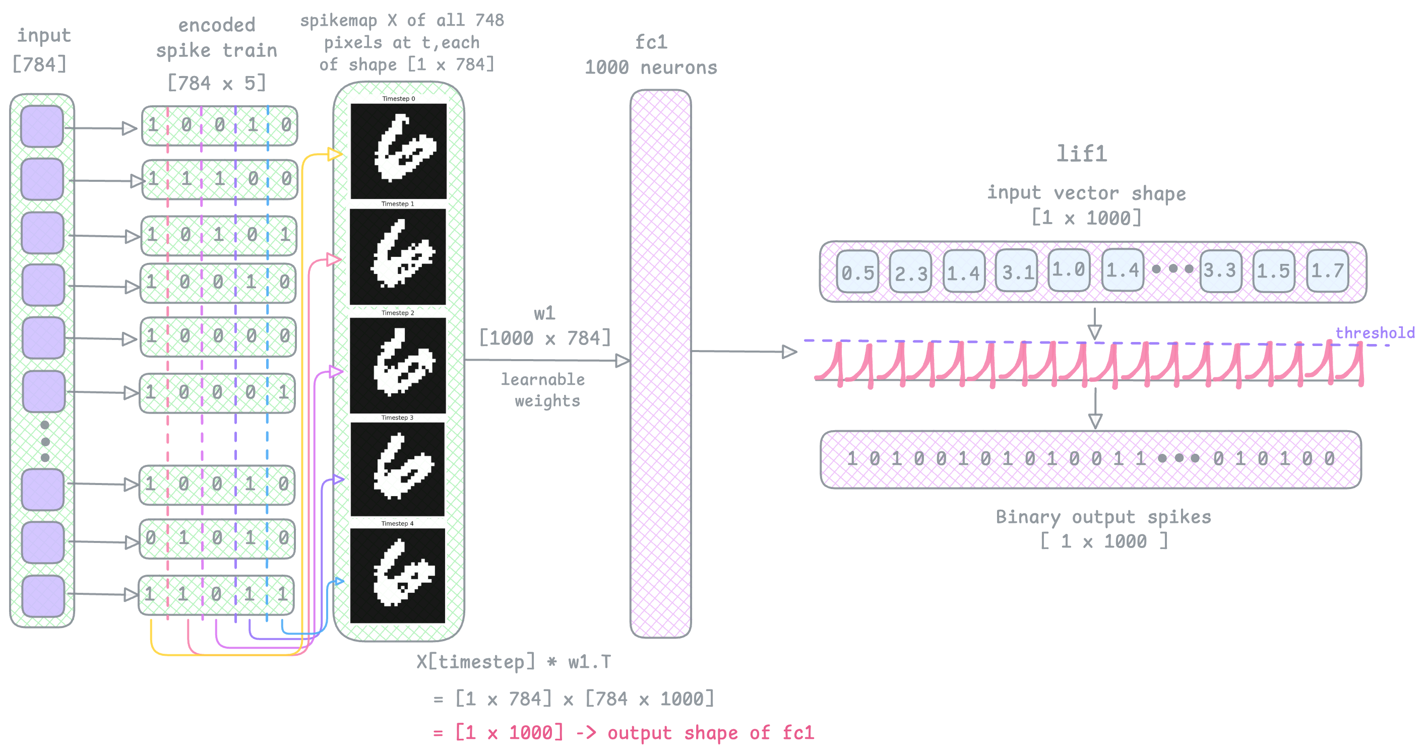
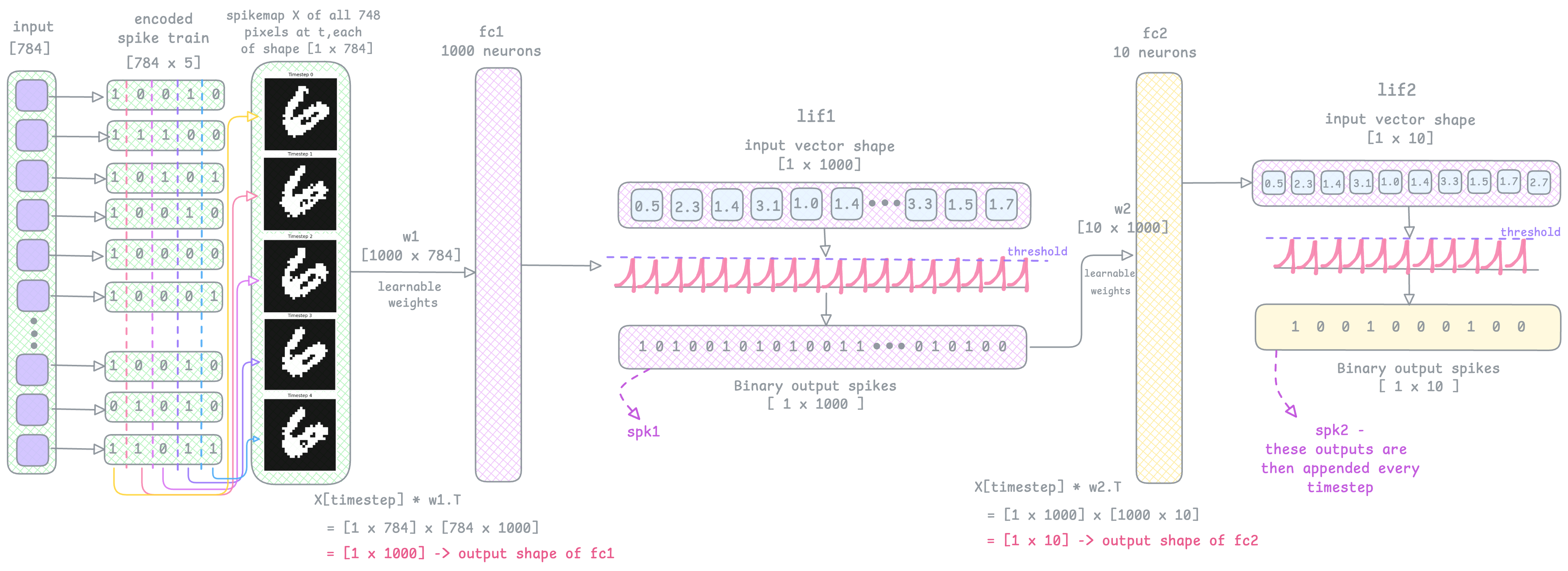
In the forward pass, we loop through each timestep. In my code I’ve used 100 timesteps so we loop 100 times. In the diagram below, I’ve shown the input image as a vector of 784 pixels, each having its own spike train of 5 timesteps long as an example.
Now, as we loop through the timesteps, at each timestep we gather all encoded spikes of that image at that particular timestep. Look at the encoded spike train layer and think of it as extracting each of its columns and gathering the bits into a spikemap (see diagram below):
This then becomes the inputs to the first fully connected layer fc1 [cur1 = self.fc1(x[step])], followed by the spiking layer lif1 [spk1, mem1 = self.lif1(cur1, mem1)]. This line of code stores the output binary spike vector in spk1 and the membrane potential values in mem1.
See the image below, the output of lif1 is an output spike train vector spk1, and this becomes the input to fc2, and then lif2.
fc2 and lif2 are the output layers, and therefore have 10 neurons (for 10 digit classification). So the fc2 layer weights w2 are of shape [10, 1000] (1000 inputs, 10 outputs).
In the above diagram & text I walked through just one timestep as an example. But this will repeat for 100 timesteps.
At the end of lif2, the output spiketrain is stored in spk2. As we loop through every timestep, we need to keep record of all output spikes spk2. This line of code does that: spktrain2.append(spk2), it appends all spk2 vectors into a list called spktrain2. At the end of the timestep loop, the final shape of spktrain2 will be [100, 1, 10], where 100 is the number of timesteps I used. Although in the image below I've just shown 5 timesteps (t=0 to t=4).
The last step of the forward pass will be to sum up all the spikes across timesteps:
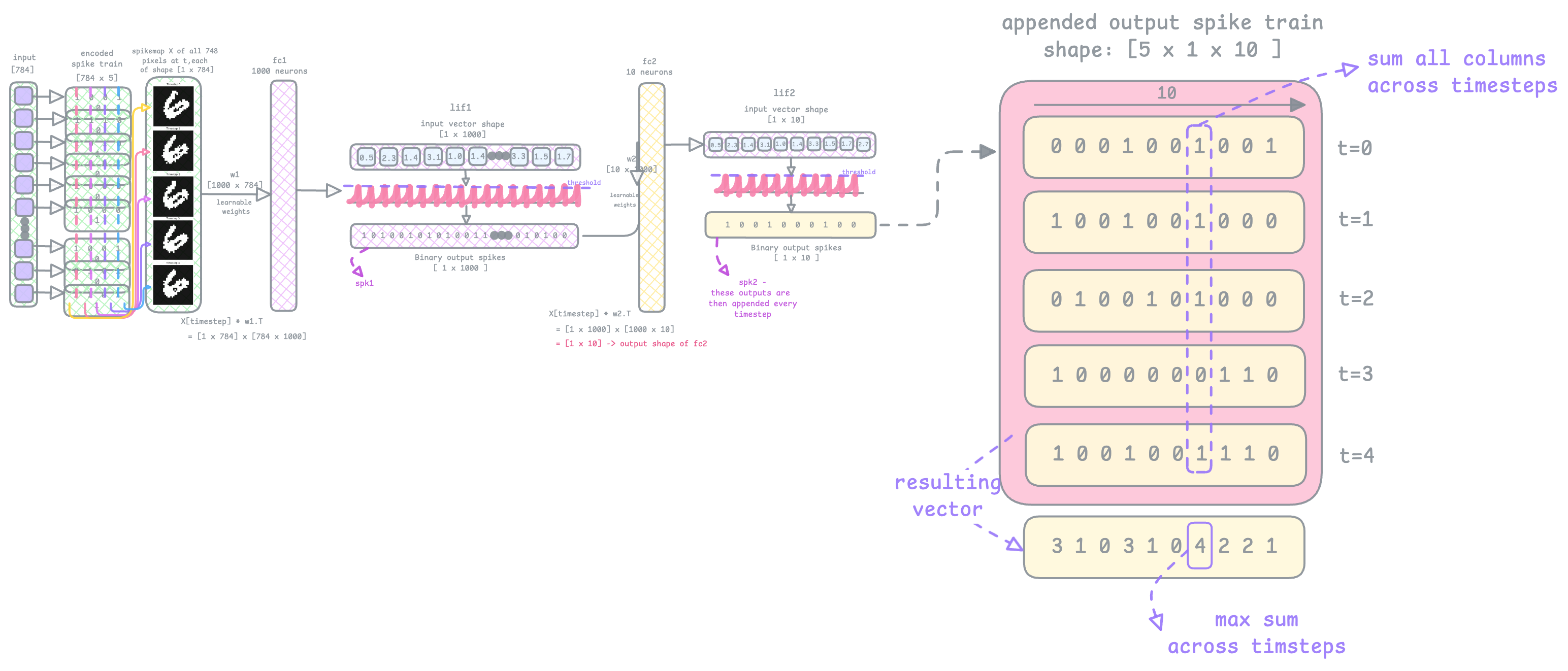
In the resulting vector you see in the image above, the 6th index has the max sum. So the predicted class is Digit 6.
This prediction is done in the line: _, pred = spkout.sum(dim=0).max(1) it sums across dim=0, and since the spiketrain2 is an appended list of all output spike trains of shape [Timestep, 1, 10] , dim=0 here is number of timesteps.
Here is the forward pass code snippet:
    def forward(self, x):
        mem1 = self.lif1.init_leaky()
        mem2 = self.lif2.init_leaky()
        spktrain2 = []
        memtrain2 = []

        for step in range(timesteps):
            cur1 = self.fc1(x[step])
            spk1, mem1 = self.lif1(cur1, mem1)
            cur2 = self.fc2(spk1)
            spk2, mem2 = self.lif2(cur2, mem2)
            spktrain2.append(spk2)
            memtrain2.append(mem2)

        return torch.stack(spktrain2), torch.stack(memtrain2)
This is a plot of all spikes through the layers:
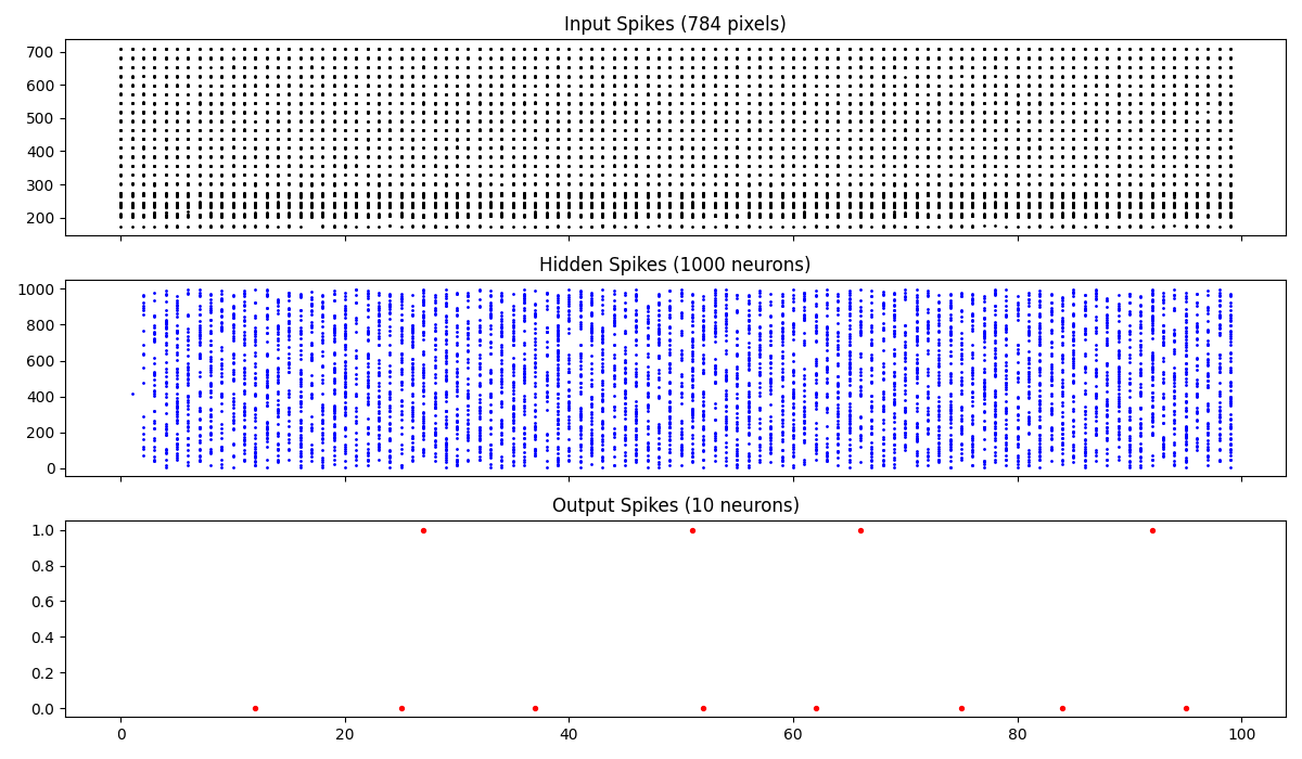
Some more explanation on what you’re seeing here: The top most map shows which input pixels out of the 784 input image pixels (y axis) spike at each of the 100 timesteps (x axis). Notice the darker band at the bottom at 200-300 pixel range - its darker because pixels that are brighter will spike more frequently.
In the hidden layer, the model recognizes patterns in the input spike trains. From weights w1, each weight indicates how much importance to give each input spike. So when we see strong patterns like bright pixel intensities, the neurons fire (spike) faster by reaching the membrane potential threshold faster.
In the last output layer, you can see most of the spikes aligned horizontally around 0. This means that the predicted digit is most likely 0.
Learning through Patterns, Frequency and Timing
In SNNs, very much like the brain, the network is trying to see when the patterns are occuring. Chances are that a neuron could only fire once in all of 100 timesteps (cause of darker pixel intensities, and low stimulus for the brain causes less firing). But a neuron firing at t=10 could have more impact than a neuron firing at t=90, because early spikes suggests to the model that there is a more immediate response to the stimulus.
The model understands how strong the evidence of a class is through frequency of spikes (how many spikes have occured in one spike train). For example if a particular group of hidden neurons spikes early, more frequently, and in a curved spiking pattern then plausibly the predicted class is Digit 6.
Over time, the model recognizes the pattern of spiking, certain neurons associated with the brighter pixels (1s) will send spikes consistently over 100 timesteps, at a certain frequency, which is how the model learns.
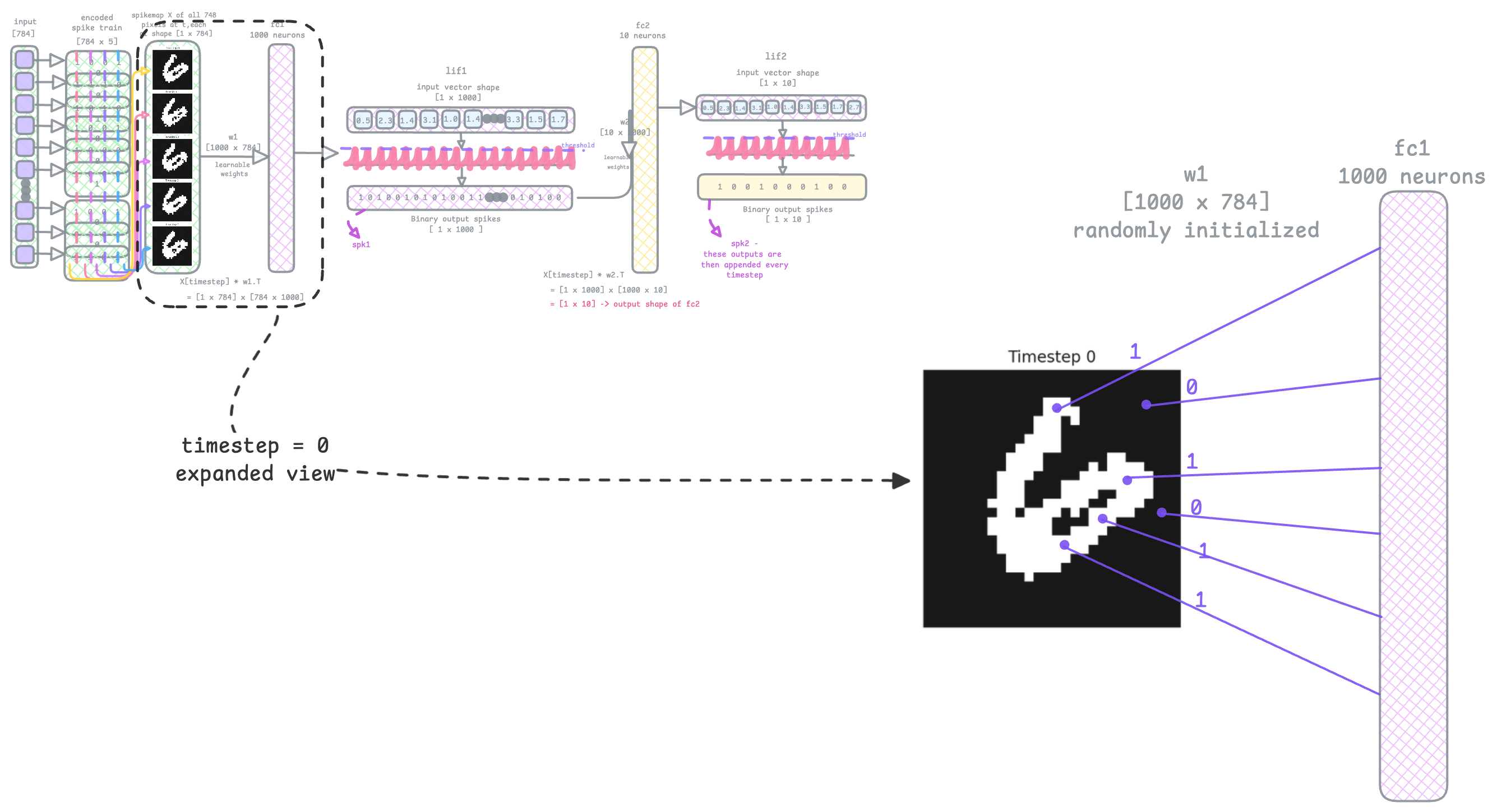
Look at the image above. The input is a rate encoded spike map at t=0, (NOT the static input image from the dataset), which is a [1 x 784] vector of 1s and 0s. Lets assume only 100 pixels spiked (the 1s - from the brighter pixel area). There are 784 inputs in total, and each input is multiplied with its weight. The 0s coming from the dark pixels have no contribution because when mulitplied with its weight, the resulting value gets zeroed out anyway. So only the bright pixels contribute.
This is where SNNs help keep the model sparse & reduce computational energy.
Learning Synaptic Weights (Backprop!)
Surrogate Gradients
SNN backprop is different. We cannot compute gradients at each layer like we do in traditional neural lets because SNNs pass down spikes, and spikes are non differentiable because they are discrete binary (1 or 0) values. When we call the LIF layer in the forward pass
(spk1, mem1 = self.lif1(cur1, mem1)), snnTorch uses a Heaviside step function under the hood to compute the output binary spikes. The gradient of this step function is infinite at the threshold and 0 everywhere else, which creates a dead neuron problem because there is no learning anywhere. So now there is no way to signal / reward based on how close you are to the target.
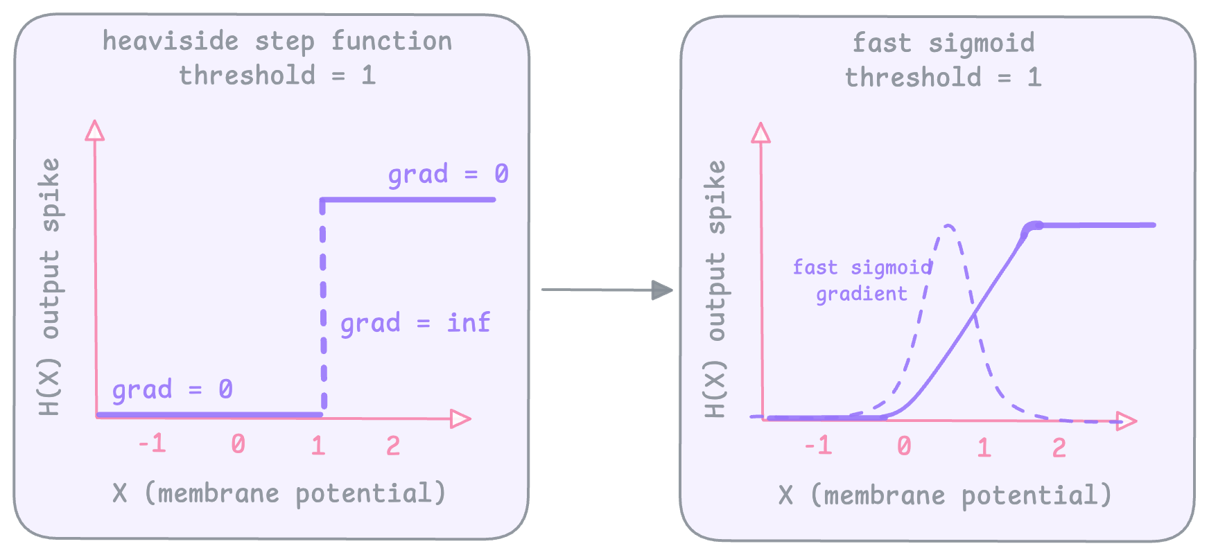
To fix this we use surrogate gradients to smoothen out the heaviside function and get gradients during backrop. When you call backward() in snnTorch, by default it uses an ArcTan function as the surrogate. But the idea is you can use any smooth curve that will result in non zero gradients (sigmoid, fast sigmoid, arcTan etc).
This surrogate gradient method is however not really brain inspired. It is just replacing a discontinuous function to continue backpropagating like in regular neural networks. To mimic the brain we need to consider the timing of spikes while learning.
Spike Timing Dependent Plasticity
Earlier in the blog I introduced the term synaptic plasticity as a neurons ability to change its synaptic strength (weights) over time, and this is based on the timing of input and output spikes. Hebbian learning says that when output spikes consistently occur after the input spikes, the synaptic weights strengthen because clearly the output spikes are caused by the input, but if output spikes occur regardless of the input spikes, then the weights weaken because the inputs are not really contirbuting to the output spiking.
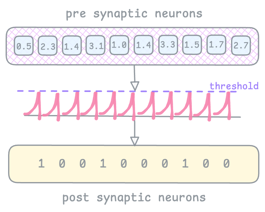
How I understand this is: I showed you earlier how we perform matmul between spike encoded inputs and weights from fc1 layer, and this weighted inputs are sent to the LIF1 layer to be accumulated, integrated and fires output spikes. So pre synaptic neurons (input spikes) must have accumulated (contributed) enough to cause an output spike, in that case, that particular weight can be nudged.
In my code however I have used surrogate gradients to train the network because snnTorch does not seem to have documentation or support for STDP as of now.
Computing Power Efficiency of the model
Let's see how much more power efficient this SNN model we just implemented is compared to a traditional ANN. For refernce, I took the computation from this paper. Due to hardware restrictions, we would have to compute this manually. But the math is simple so it’s okay.
First, for the SNN compute synaptic operations and energy per layer using the formula:
SOPs per layer: SOPs = T × γ × FLOPs
where T is the number of times step required in the simulation, γ is the firing rate of input spike train of the layer, and FLOPs is the estimated floating point operations at that layer.
SNN energy per layer: \(Power_{SNN} = 77\text{ fJ} \times \text{SOPs}\)
> (77 femtojoules is energy consumed per synaptic operation)
The formula for an ANN,
ANN energy per layer: \(Power_{ANN} = 12.5\text{ pJ} \times \text{FLOPs}\)
> Note that 1J = 103 mJ = 1012 pJ = 1015 fJ.
To find \(\gamma\) I wrote this script to compute using the formula:
\[\gamma = \frac{\text{Num of possible spikes}}{\text{Num of spikes observed across all timesteps}}\]
Number of possible spikes = Batch size x Number of neurons x timesteps
FLOPs per layer:
- fc1 → 784 * 1000 = 784,000
- fc2 → 1000 * 10 = 10,000
Firing rates (from code result):
- γfc1 = 0.200621
- γfc2 = 0.124000
SNN SOPs:
- $SOPs_{fc1}=$ 100 * 0.200621 * 784,000 = 15,729,726
- $SOPs_{fc2}=$ 100 * 0.124000 * 10,000 = 124,000
- total SOP = 15,853,726
SNN energy:
- $Power_{SNN}=$ 77fJ × 15,853,726 = 1,220,739,902fJ = 0.00122mJ
ANN energy:
- $Power_{ANN}=$ =12.5pJ × 794,000 = 9,925,000pJ = 0.00993mJ
Energy Reduction:
- $\text{Reduction} = \frac{0.00993}{0.00122} \approx$ 8.1x
This means the SNN implementation is ~8x more energy efficient than an ANN model!
So WHY does this work?
> Time!
What we did now is take a neural network and slap a time dimension on it to give it short term memory, and called it SNN. Having memory now means each LIF neuron can remember past inputs as it integrates its membrane potential, which is a huge part of building a brain. Our brain does not take in a static image to recognize / classify it, instead it continuosly integrates signals over time within a matter of few milliseconds.
And if you look closely, SNN is secretly just a recurrent neural net but with spikes, and a discontinuous activation (heaviside) function.
Neuromorphic Hardware
This will be a very brief overview of neuromorphic hardware. Neuromorphic computing at scale is currently being bottlenecked by Von Neumann hardware architecture, and all computers both CPU and GPU that we use follow this Von Neumann design:
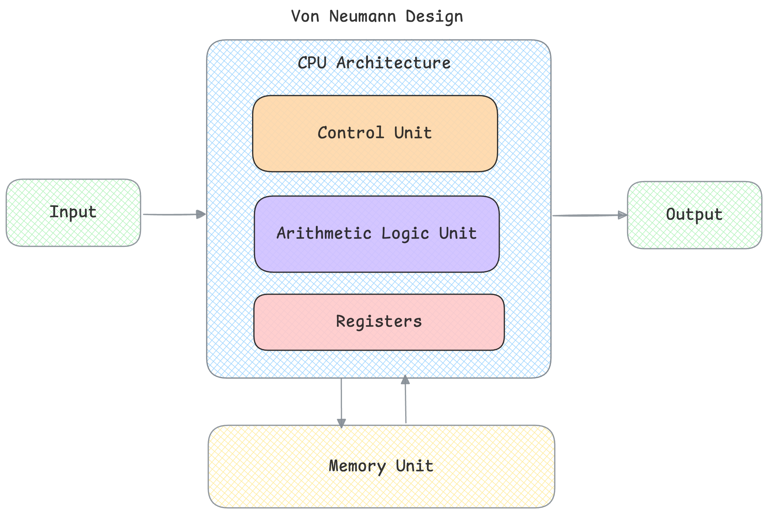
The problem with this is it is not very power efficient because the memory unit and computational unit are physically seperate, so shuttling data between cpu and memory for each computation costs time and energy. It takes about 100x more energy to move even 1 bit from DRAM than a single FLOP.
To fix this bottleneck, neuromorphic hardware combines both computation and memory into the same unit.
Moore’s Law applies here -

For decades, we’ve seen how packing more transistors in a single chip can increase computation, and Dennard Scaling showed how smaller transistor sizes requires less energy. But this will not scale anymore. It is not an option now to lower voltage simply by reducing transistor size further. And packing few more billion transistors in GPUs will still waste energy just shuffling data.
Another reason why we need seperate hardware is that SNNs are event driven, and do not process everything on a syncronized clock cycle. CPU and GPU both work on a timed clock cycle. By removing this syncronization, the idea is to save a lot of power because why perform computation for neurons that are not contributing? in SNNs, neurons only communicate when they spike, and there is no energy spent if there is no neuronal activity. So there is a need for hardware that does not force computation at every clock cycle.
A working hardware solution is on-chip routers that send spikes to specific neurons without waiting for clock cycles.
Conclusion
In this blog, we walked through how SNNs work step by step by training one on the MNIST dataset, and computed the energy efficiency of the model to be 8x more efficient than a traditional ANN. And if there's one thing you can takeaway from the blog it should be the importance of temporal dynamics in building brain inspired models.
I hope this was useful and I hope my illustrations helped you visualize SNNs! You can find the full training code in my GitHub.