Optimizing a Layer Normalization Kernel with CUDA: a Worklog
Layer normalization is a data preprocessing technique used in deep learning to stabilize training data. When we train a neural network on a dataset, most of the time, the data is on different scales. For example, let’s take a dataset of employees at some company, where the two input features are age and salary. Age data ranges from 20-50 while salary data can range from 50,000 to 100,000. Totally different scales. Normalizing helps the input features be at the same scale.
In this blog, I will iteratively optimize a layer normalization kernel written in CUDA, from scratch, by learning and using GPU optimizing techniques including memory coalescing, shuffling and vectorized loading. Let’s see if we can beat PyTorch’s implementation of layer norm. I’m using NVIDIA GeForce RTX 4050 GPU for this implementation. You can find full code in my GitHub.
This is meant to be a fun, code along blog. Let’s get started!
Layer Norm Math: Under the Hood
The math for layer norm is fairly simple. We calculate the mean $\mu$ and variance $\sigma^2$ for each input feature $X_{ij}$ sequentially. Consider each row of a matrix $X$ to be a feature. Layer norm ensures each feature has a mean of 0 and variance of 1. A very small value $\epsilon$ is added to prevent division by zero. The formula is as follows:
To compute mean and variance for each row, we apply the formulas:
Visually, assume a 3x3 input matrix:
To calculate the layer norm on the first row \(X_{row1} = [1,2,3]\), find the mean, variance and normalize like so:
Similarly, compute mean, variance and layer norm for every row to achieve the following output matrix. Throughout this worklog, assume epsilon $\epsilon$ to be $10^{-6}$.
PyTorch Benchmark
To begin, let’s see how fast a layer norm implementation is in PyTorch for a 1024 x 1024 matrix. We will use this same input dimension for all kernels.
    import torch
    import torch.nn as nn
    import time

    m, n = 1024, 1024
    # input matrix is 1,2,3,4...1048576
    input = torch.arange(1, m*n+1).reshape(m,n).float()

    # LayerNorm
    layer_norm = nn.LayerNorm(n, elementwise_affine=False, eps=1e-6).cuda()

    #warm up GPU
    for i in range(10):
        output = layer_norm(input.cuda())


    # measure time
    start = time.time()
    for i in range(1000):
        output = layer_norm(input.cuda())
    torch.cuda.synchronize()
    end = time.time()

    pytorch_time = (end - start)/1000
    print(f"PyTorch LayerNorm time: {pytorch_time * 1000:.4f} ms")
Output:
PyTorch takes around 0.4 ms to compute layer norm on a 1024 x 1024 matrix.
PyTorch LayerNorm time: 0.4447 ms
Kernel 1: Naive Layer Normalization
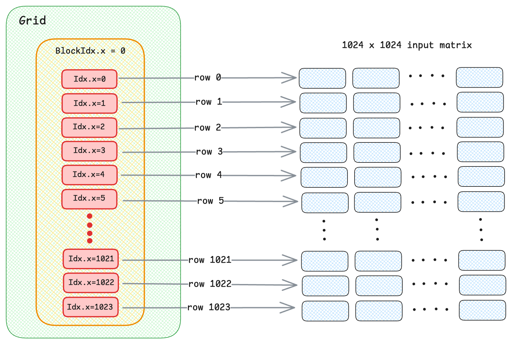
The first kernel is going to be a naive implementation, where we replicate the formulas shown in the example above. For this approach, one thread in a block normalizes one row. When we invoke the kernel with __global__, the execution launches a grid of threads where each thread processes a single row of the input matrix.
This line of code assigns the row index that the current thread will process.
int row = threadIdx.x + (blockDim.x * blockIdx.x);
Once the threads are assigned to its rows, there are three stages to the layer norm computation - mean, variance, and putting them both together to find the norm. Let’s analyse the three loops.
- Loop 1: The thread loops over all elements in its assigned row. It reads each element from global memory and accumulates the sum. The sum is then divided by n total number of columns to find the mean.
- Loop 2: The same thread loops through the row again, this time to compute variance.
- Loop 3: Finally, the thread loops through the row again, subtracting the mean and dividing by the standard deviation - which is the square root of variance.
Normalizing code:
    // compute mean
    for(int col = 0; col < n; col++){
        int idx = row * n + col;
        mean += X[idx]; // reading from global memory
    }
    mean /= n;

    // compute variance
    for(int col = 0; col < n; col++){
        int idx = row * n + col;
        var += (X[idx] - mean) * (X[idx] - mean);
    }
    var /= n;

    // normalize each row
    float stddev = sqrt(var + EPSILON);
    for(int col = 0; col < n; col++){
        int idx = row * n + col;
        P[idx] = (X[idx] - mean) / stddev;
    }
As you may notice, at each for loop, the thread reads each element from global memory X[idx]. Which means that the thread accesses the input row from global memory three times, causing high traffic. We will learn how to optimize this in the next kernel.
Since we have 1024 rows, we need 1024 threads per block and m + threadsPerBlock - 1. We can launch our kernel as:
    dim3 threadsPerBlock(1024); // 1024 rows
    dim3 blocksPerGrid((m + threadsPerBlock.x - 1) / threadsPerBlock.x);

    // kernel launch
    naive_layernorm<<<blocksPerGrid, threadsPerBlock>>>(D_in, D_out, m, n);
The kernel performance is as follows:
Naive Kernel Execution time: 2.3886 ms
As expected, this naive implementation is around 2 ms slower than PyTorch. Let's do better.
Kernel 2: Shared Memory Reductions and Coalescing
In this kernel, let’s walk through how to reduce frequent global memory access by using shared memory instead.
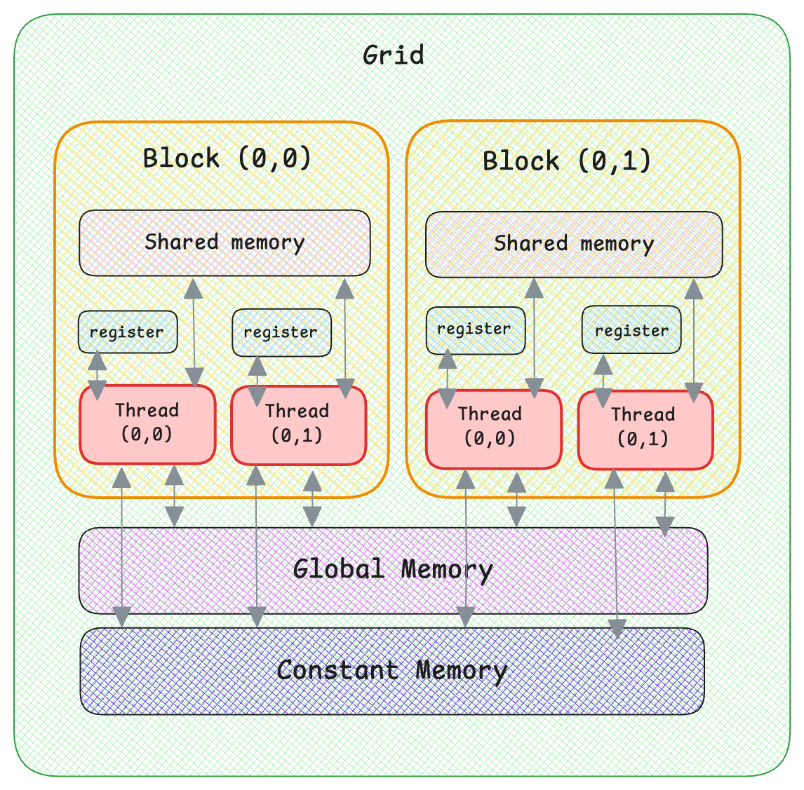
In GPU memory architecture, it is faster to access shared memory due to lower latency. Each block has its own shared memory and all threads in a block can access the same shared memory. And all blocks can access the same global memory. Each thread has access to its own unique register.
For this implementation, let’s assign one block per row (as opposed to one thread per row in naive kernel).
These lines of code do that for us:
    //one block per row
    int row = blockIdx.x;
    int tidx = threadIdx.x;
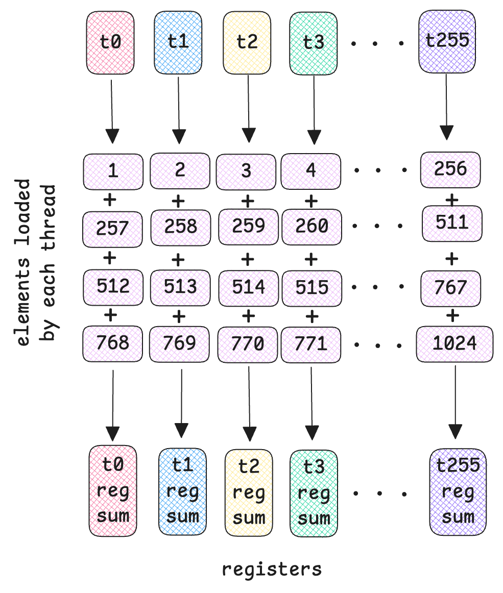
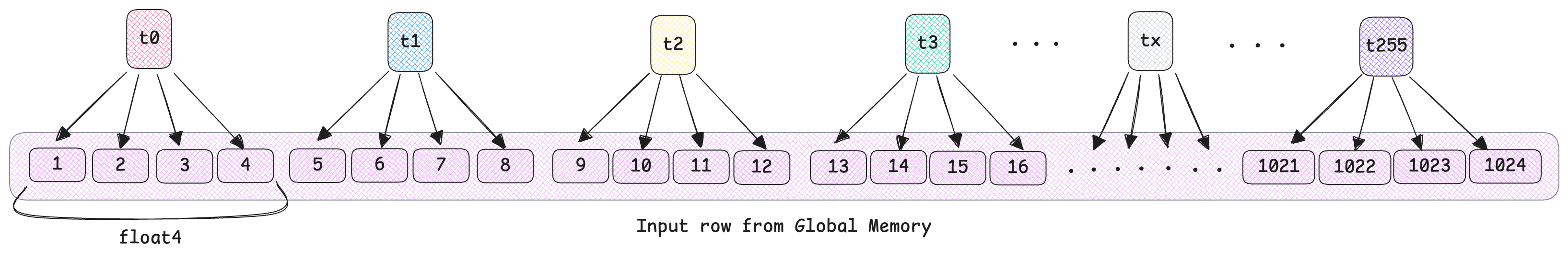
A more efficient way to load from global memory is to use memory coalescing. Which is to have consecutive threads access consecutive memory addresses.
Take a look at the diagram below. We will be using 256 threads per block. So threads t0 - t255 will load consecutive elements 1-256. In the second iteration, threads, t0 - t255 will then load consecutive elements 257-511 and so on, until each thread in our case, has loaded 4 elements spaced by blockDim.x = 256.
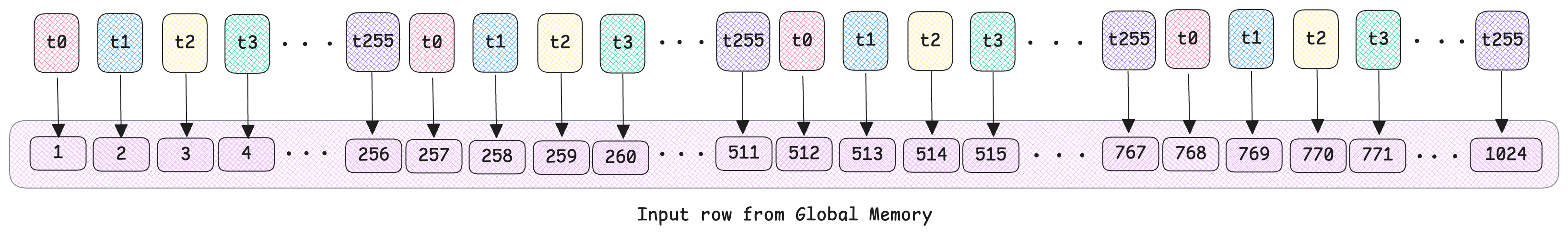
Note that this diagram illustrates one input row, there are m = 1024 of these blocks that process each row of the input.
This is done in the following code snippet:
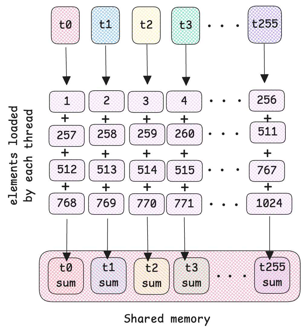
    for(int i = tidx; i < n; i+=blockDim.x){

        float a = row_in[i]; // load from global mem into register
        lmean += a; //sum for now
        lvar += (a*a);
    }

    smem[tidx] = lmean; // contains the sum of all values loaded by that thread tidx
Each thread accumulates the sum of the elements it loaded and stores it in shared memory smem.
Now that we have all the local sums, it’s time for reductions. We need to find the total sum of all elements in the shared memory so we can compute its mean. This is done in log(n) steps as we reduce hierarchically. Eventually, the global sum ends up in the first index smem[0] of shared memory. In the example below, assume the 8 random values are the local sums each thread just computed. This diagram below explains reductions:
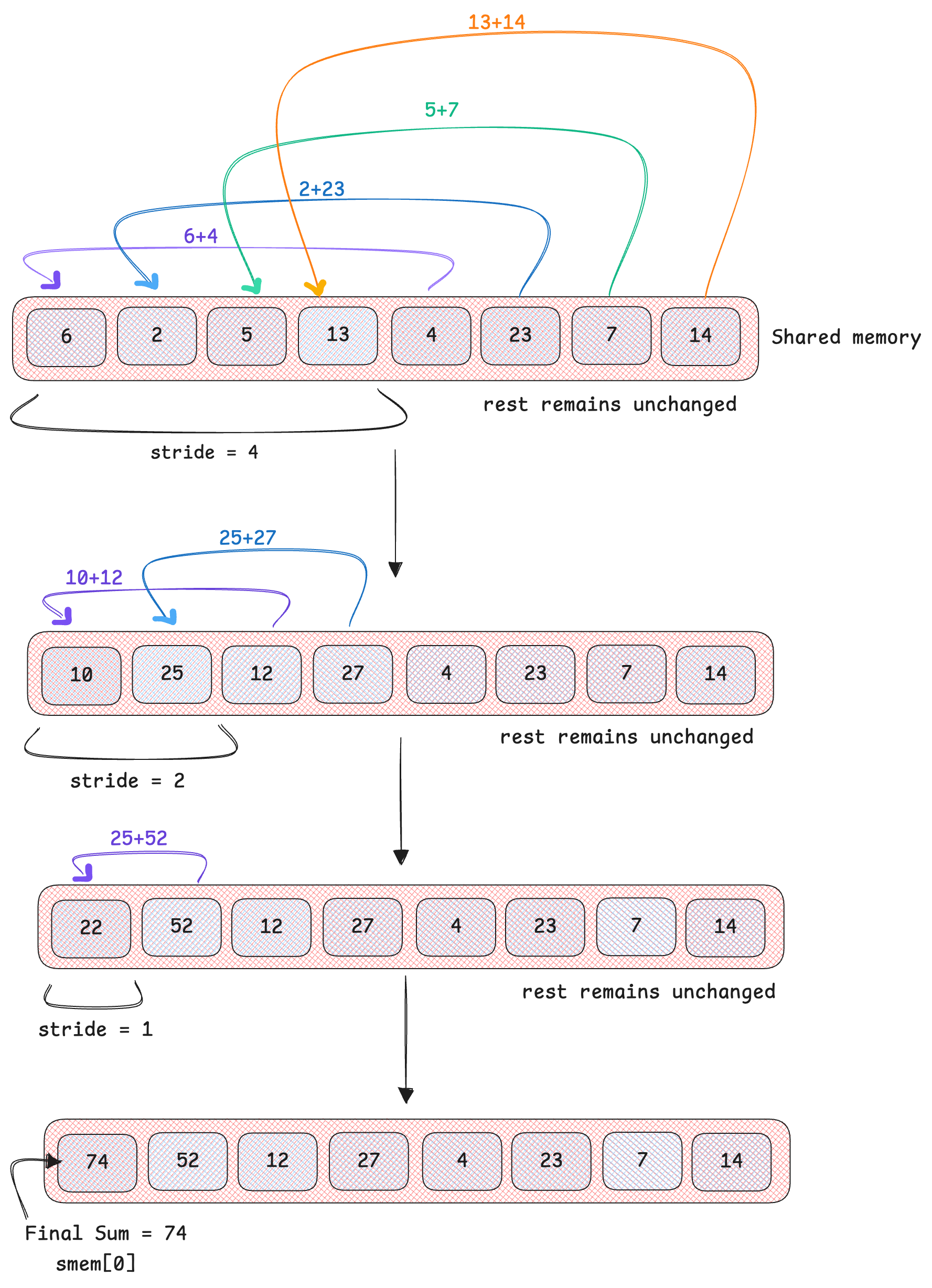
stride begins as half of blockDim.x, and is halved as we iterate. The thread elements within the first stride are added to the thread elements in tidx + stride (tidx is thread index).
As you can see, the final sum accumulates at the first index of our shared memory. We can then take that value and divide by n to compute global mean for each row, followed by the global variance similarly. This code snippet performs reduction:
    for(int stride = blockDim.x / 2; stride > 0; stride /=2){
        if(tidx < stride){
            smem[tidx] += smem[tidx + stride]; // the sum will end up in index 0
        }
    }
    float gmean = smem[0] / n;
Once we have our global mean and variance values, we can finally compute the layer norm.
    // normalize and store outputs
    for(int i = tidx; i < n; i += blockDim.x){
        row_out[i] = (row_in[i] - gmean) * stddev;
    }
Each thread tidx normalizes and stores its assigned elements and writes back to global memory row_out[i] in a coalesced manner.
The output performance of this kernel is:
Reduction Kernel Execution time: 0.08168 ms
We are already more efficient than PyTorch! But we can still do better.
Kernel 3: Warp level Shuffle functions
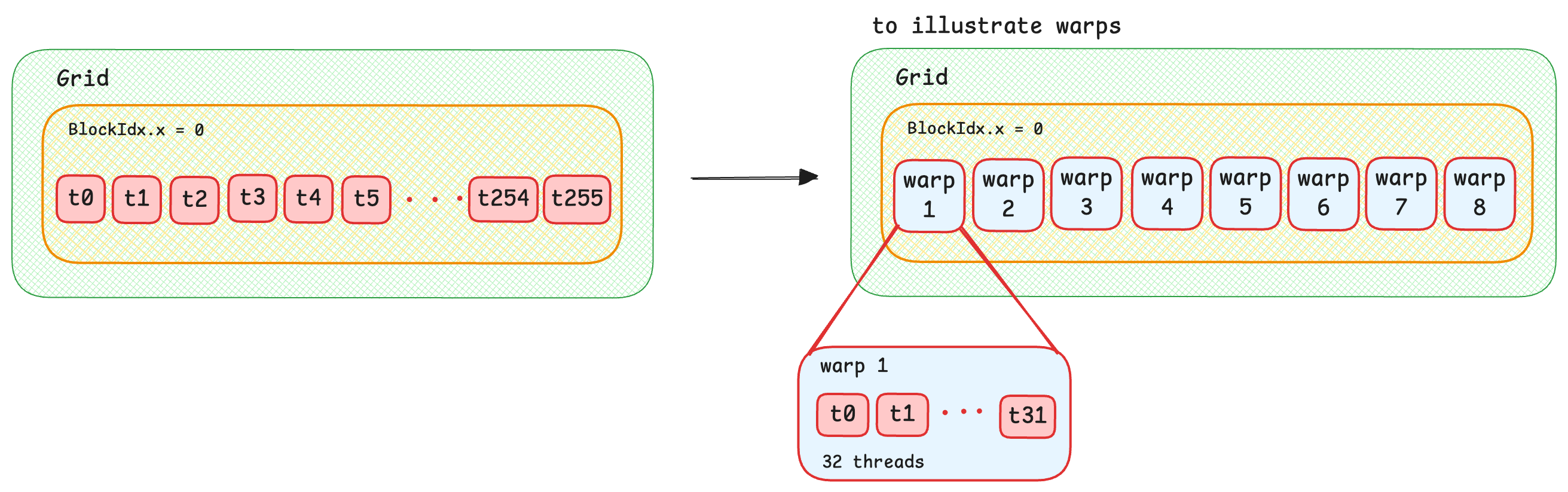
We made it to kernel 3! For this implementation, let’s further optimize by using registers at the warp level instead of shared memory. If you recall the GPU memory architecture, you can see that accessing registers is faster than accessing shared memory.
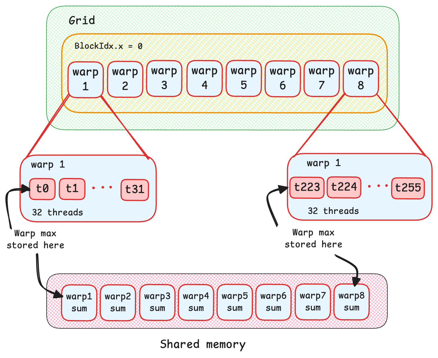
In GPU programming, warps are a group of (usually 32) threads that are executed in parallel. In our case, we use 256 threads per block, so number of warps = blockDim.x / warp_size = 256/32 = 8 warps per block.
Similar to kernel 2, we load the input values from global memory into registers using memory coalescing.
    for(int i = tidx; i < n; i += blockDim.x){
        float a = row_in[i];
        lmean += a; //lmean is just the sum for now (will divide later)
        lvar += (a*a);
    }
    __syncthreads();

    // store in register instead of smem
    float lrmean = lmean;
The only difference from kernel 2 is, instead of storing local sums into shared memory (smem[tidx] = lmean)❌, we store it in the thread’s register (float lrmean = lmean)✅ and use shuffle functions to pass the values across threads in a warp. Don’t worry, let’s see what that means.
Warp Level Shuffling
Similar to how we used strides in kernel 2, to stride across shared memory and perform sum reduction, we are going to stride across warps in a block to find the sum of each warp, again in a log(n) manner. Here is everything you need to know for warp level shuffling:
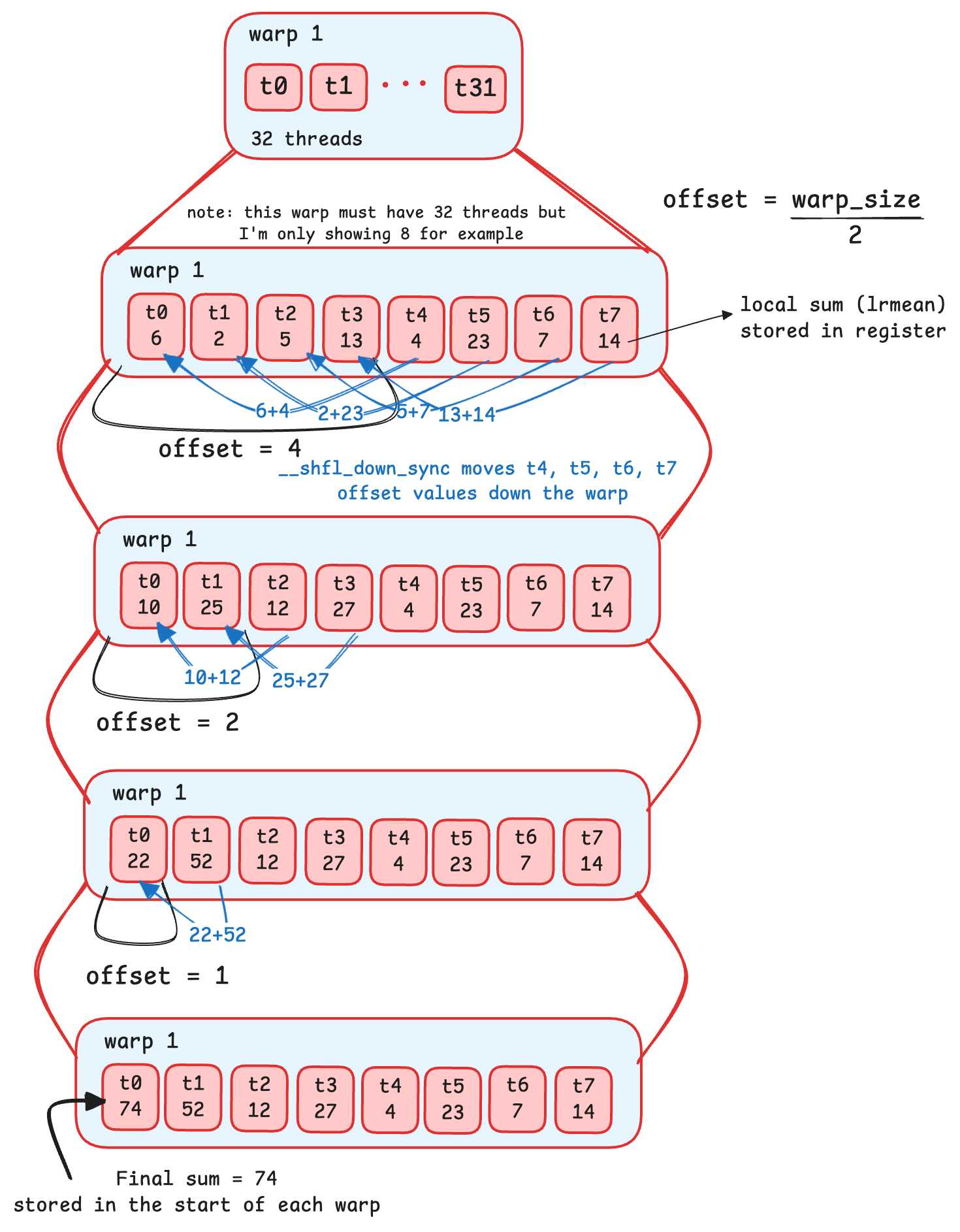
As you can see, __shfl_down_sync is responsible for moving values down a warp by offset values. At the end of the loop, the final sum (within that warp) is stored at the first index. In the drawing I’ve only 8 threads in a warp for example, but there are 32 doing this operation. 0xffffffffsets the range to all threads in the warp.
Here is the code for that:
    // global mean, warp level using shuffling
    for(int offset = warp_size/2; offset > 0; offset /= 2){
        lrmean += __shfl_down_sync(0xffffffff, lrmean, offset);
    }
    // at this point, each warp finished summing values at each warp
    // sum of each warp is stored at 0 index of each warp
Next, we need to repeat that process for all warps in a block. Since we are using 256 threads per block, we have 256/32 = 8 warps to reduce. Once reduced, all warps will have stored its total sum for that warp at its first index. We can then save those sums from each warp into shared memory, which will later be reduced further.
    // global mean, block level using shuffling
    if (blockDim.x > warp_size){
        if(tidx % warp_size == 0){ // if first index of a warp
            smem[tidx/warp_size] = lrmean; //store sum of each warp into smem
        }
Block level shuffling
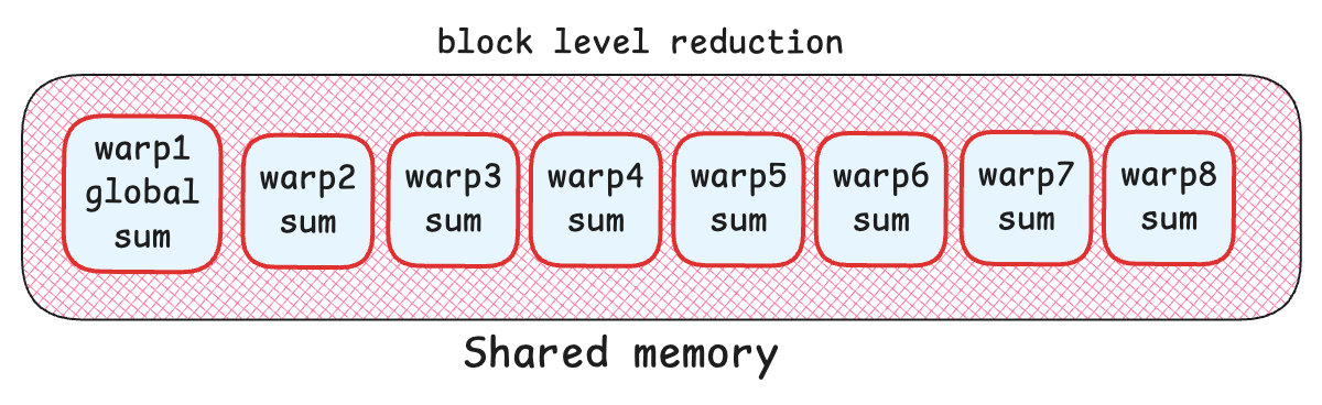
Next, we need to reduce the warp sums that we have stored in our shared memory. This will give us the global sum of the entire row. To do this, we only need the first warp of threads to load warp sums from shared memory to further reduce the sums. We set the other thread values from other warps to 0. Once again, we perform warp reduction using __shfl_down_sync and at the final iteration, lrmean will have the final sum (the sum of the entire row). Finally, divide it by n to get the gloabal mean.
    if(tidx < warp_size){ // only first warp
        // load from smem to warp, set other warps to 0.0
        lrmean = (tidx < (blockDim.x + warp_size - 1) / warp_size) ? smem[tidx] : 0.0f;
        for(int offset = warp_size / 2; offset > 0; offset /=2){
            lrmean += __shfl_down_sync(0xffffffff, lrmean, offset);
        }

        if(tidx==0){
            smem[0] = lrmean;
        }
    }
    float gmean = smem[0] / n; // global mean stored at first index of smem
So far, we computed global mean using warp level and block level reductions of the entire row. Now we need to repeat warp and block reductions to find the global variance of that row.
Finally, the global sum will then be stored at the first index of shared memory, which is used to find global mean and variance.
Code snippet for computing global variance:
    // local variance
    float lrvar = lvar;

    // warp level reduction
    for(int offset = warp_size/2; offset > 0; offset /= 2){
        lrvar += __shfl_down_sync(0xffffffff, lrvar, offset);
    }

    // block level reduction
    if (blockDim.x > warp_size){
        if(tidx % warp_size == 0){
            smem[tidx/warp_size] = lrvar; // storing local warp variance in smem
        }
        __syncthreads();

            // using only first warp
        if(tidx < warp_size){
            lrvar = (tidx < (blockDim.x + warp_size - 1) / warp_size) ? smem[tidx] : 0.0f;
            for(int offset = warp_size / 2; offset > 0; offset /=2){
                lrvar += __shfl_down_sync(0xffffffff, lrvar, offset);
            }

            if(tidx == 0){
                smem[0] = lrvar;
            }
        }
    }
    else{
        if(tidx == 0){
            smem[0] = lrvar;
        }
    }
    __syncthreads();

    float gvar = (smem[0] / n) -  (gmean * gmean); // Load global variance
This kernel outputs:
Shuffled Kernel Execution time: 0.07261 ms
We are now 10% faster than kernel 2! Let's go a little further.
Kernel 4: Vectorized Loading
For our final kernel, let’s try to optimize this further by making our memory access even more efficient. So far, in our coalesced implementations, one thread loads one element at a time from global memory into registers and accumulates the sum at each iteration. Instead, what if we load 4 elements per thread? This is called vectorized loading.
We divide the total number of elements in a row by 4 to get the total number of vectorized iterations: vect_iters = n/4
Here we have 1024/4 = 256 vec_iters. Since we have 256 threads, each thread will load 4 elements at the same time. Each thread loads float4 values at once. See diagram above.
    int vec_iters = n / 4;
    for(int i = tidx; i < vec_iters; i += blockDim.x){
        float4 v = reinterpret_cast(row_in)[i];
        lmean += v.x + v.y + v.z + v.w; // div by n later for mean
        lvar += (v.x * v.x) + (v.y * v.y) + (v.z * v.z) + (v.w * v.w);
    }
float4 is an in-built struct, so we can access the four elements v loaded by v.x, v.y, v.z, v.w. So in each iteration, one thread loads 4 elements and sums them to compute local mean and variance. Much more efficient than coalescing.
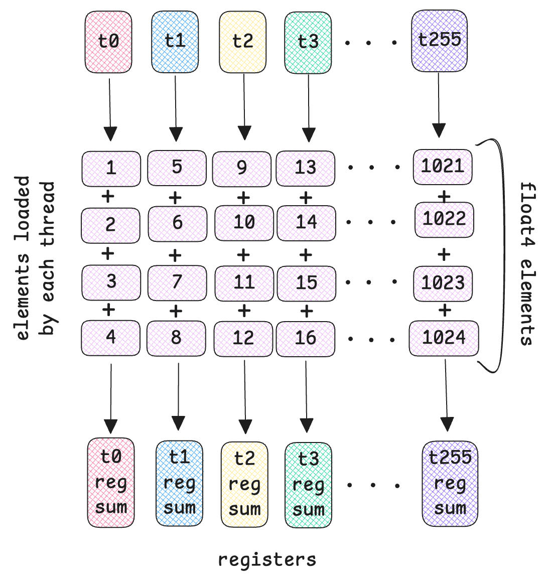
Pay attention to the values loaded by the threads here. It’s different from the previous kernels. The sum of float4 elements are stored in the threads personal register. And now we can perform warp level reduction using __shfl_down_sync on these threads to find the global mean and variance.
The warp reduction code is the same:
    // reducing sum across warps
    for(int offset = WARP_SIZE / 2; offset > 0; offset /=2){
        lmean += __shfl_down_sync(0xffffffff, lmean, offset);
        lvar += __shfl_down_sync(0xffffffff, lvar, offset);
    }

    // global mean and variance
    float gmean = lmean / n;
    float gvar = (lvar / n) - (gmean * gmean);
    float std_inv = rsqrtf(gvar + EPSILON);
Finally, we can compute the layer norm. We subtract each element of float4 by global mean and divide by standard devitation. Now, we can load it back to global memory in a vectorized manner: reinterpret_cast
    for(int i = tidx; i < vec_iters; i += blockDim.x){
        float4 v = reinterpret_cast(row_in)[i];
        v.x = (v.x - gmean) * std_inv;
        v.y = (v.y - gmean) * std_inv;
        v.z = (v.z - gmean) * std_inv;
        v.w = (v.w - gmean) * std_inv;
        reinterpret_cast(row_out)[i] = v; // load to global mem
    }

    // remainder elements not included in vectors
    for(int i = vec_iters * 4 + tidx; i < n; i += blockDim.x){
        row_out[i] = (row_in[i] - gmean) * std_inv;
    }
This kernel outputs:
Vectorized Kernel Execution time: 0.05632 ms
And Yes! Our vectorized approach is around 0.35 ms faster, that is around 87% more efficient than PyTorch’s implementation of layer norm!
Conclusion
In this worklog, we saw what layer norm is under the hood, benchmarked PyTorch implementation and iteratively wrote optimized kernels from scratch. We learnt a naive implementation using one thread per row to perform all computations. We then moved on to learning to manipulate threads to perform memory coealescing, used shared memory instead of accessing global memory. We also went over warps and how using registers to access values is faster than shared memory. Finally we made loading elements faster by vectorizing loads.
The point was not to beat PyTorch’s implementation, but to learn GPU programming and optimizing techniques to make our code efficient, and parallelize repetitive patterns using our GPU.
I hope this worklog was useful and I hope my illustrations helped you visualize CUDA! You can find the code implementations for all the kernels in my GitHub.